Chapter 4
REALTIME TRANSCRIPTION OF HAND-DRUM TIMBRES
4.1 Introduction
The eventual goal of this dissertation is to develop methods that allow musical robots to learn how to use timbre by listening to humans play. This will require the robots to transcribe the timbres in human performance.
Researchers have long struggled to give a precise definition to `timbre', and in fact different researchers seem to use the word to refer to different things at different times. It is not clear whether `timbre' refers to a steady-state phenomenon or a dynamic one, whether it refers to a physical acoustic property of sound or a purely perceptual one, or whether our perception of it is innate or learned through culture. This has given rise to the often-repeated definition that timbre is the sum of all qualities of sound aside from pitch and loudness. However, one might argue that even pitch and loudness are implicated in timbre because in practice they are not always orthogonal to other features of sound. For instance, as the human voice becomes louder, it also becomes brighter [65]; the amplitude envelope of a sound is often considered a part of timbre; a given pitch on a given instrument is linked to timbre via register; etc... As has been previously noted, `timbre' comes from the Greek word `τuμπανον', indicating a small membranophone. The exact reason for this etymology is not clear, although it seems apt given the present application. Any membranophone is capable of producing a bounded but infinite variety of perceptually distinct sounds, depending on where or how it is struck or actuated. Similar statements can be made for other instruments. Within the context of this paper, the `timbral space' of an instrument shall refer to the space of all such sounds which are under control of the musician while playing the instrument. `Timbre' shall refer to a point in that space, and performance shall be understood to entail navigating that space. It shall be assumed that the timbral spaces of all membranophones are subsets of a larger, comprehensive timbral space, and it shall be further assumed that this space is metrizable. Such a space and metric shall be presented in this chapter.
There exists a common aphorism that says `data ≠ information ≠ knowledge ≠ wisdom'. It is generally true that raw features only go so far in characterizing the phenomenon they measure. For instance, it is common for designers of new musical interfaces to make synthesizers with continuous orthogonal control of raw timbral parameters (data) such as brightness and noisiness. The inverse approach could easily be taken in transcribing timbre from a performance, by tracing a performer's trajectory through a raw timbral feature space. However, such features have little higher-level meaning. At the `information' level in the hierarchy, timbre is often considered a discrete phenomenon. Iconic sounds such as a heavily distorted electric guitar or a violin playing sul ponticello have socially constructed semiotic meanings [66]; sul ponticello is used in particular contexts within particular genres to convey particular musical ideas. However, sounds like these are not single points in a raw feature space; there is a certain variability in the bowing method that will produce a recognizable sul ponticello timbre. More properly, these sounds are regions in a timbre space. If the semiosis of timbre is of interest, it might not be important to know the raw numerical values of the features that characterize these sounds; it may only be important to know whether a given timbre lies in a particular discrete region. One challenge with representing timbre discretely is that the regions of interest may not be known in advance. Here, machine learning provides a solution that allows a human musician to specify the regions of interest by playing examples of the corresponding timbres.
In the case of membranophones, players generally define a finite number of methods of striking the drum (strokes), each with a characteristic, discrete timbre. This is especially true for drums that are played with bare hands. In general, rhythmic patterns on these instruments are largely defined by the sequence of timbres that comprise them. Therefore, in order to transcribe such a rhythm, one must know which strokes were used to articulate it. In the case of a percussion robot, if the robot is to `learn' rhythms from the human by modeling the musical context of different timbres, it will be simplest if the human is playing an instrument whose technique is similar to the robot's. For this reason the following study focuses on timbre classification using percussion instruments that are played with the hands (such as djembe or cajon) as opposed to sticks (such as snare drum), and whose strokes are not characterized by subtle manipulations of the fingers (such as tabla).
4.2 Previous Work
Exhaustive studies have been successful at classifying percussive sounds [67,68]. Such studies seek to grossly identify the instrument that produced the sound, but the present goal is to identify more subtle timbral nuances within a single instrument. The feature sets in those studies are also quite large, so another present goal is to use a smaller feature set that can be implemented to run efficiently in real-time. This will also reduce the volume of the feature space so that fewer training examples may be used. Hochenbaum and Kapur [69] detect nuances in a percussionist's playing via an accelerometer on their wrists. In their seminal robot Haile, Weinberg and Driscoll [47] use fundamental frequency estimation to estimate where (radially) a human strikes a large `pow-wow' drum. The work presented in Section 4.3.2 below suggests that this one feature is not sufficient to categorize sounds in the current application. Sarkar [70] and Chordia and Rae [71] evaluate several methods for classifying tabla strokes, which are characterized by subtle digital manipulations. Tindale, Kapur and Fujinaga [72] perform a study similar to the present one focused on snare drum, which is played with drumsticks. Although both [70] and [72] are intended to be realtime, they both operate upon a few hundred milliseconds of audio, which limits the maximum speed of playing to a few Hz. The current study presents a full, working realtime implementation for hand drums that does not limit the player's repetition rate.
4.3 Implementation
4.3.1 Onset Detection
In order to classify strokes in realtime, it is first necessary to detect where in the signal the strokes occur. In the current context (a contact-mic affixed to a single percussion instrument), even the most naive onset-detection algorithm, such as amplitude thresholding, would likely suffice for a laboratory experiment. However, a more robust algorithm was implemented here - a variant of the one described in [73]. Specifically, an STFT is performed on the incoming audio stream. At each analysis frame, the bins are identified whose magnitudes have increased since the previous frame, and the amount of positive change is accumulated over all of the bins. The resulting values, computed at each successive analysis frame, serve as an onset-strength signal (OSS). Noise is removed from the OSS by low-pass filtering. Percival uses a 14th order filter which will introduce a delay of 40 milliseconds at a sample rate of 44.1 kHz. In order to minimize this delay, in the current implementation the filter-order was hand-tuned to the lowest acceptable value, 4, resulting in 12 ms delay. Peaks are picked from the OSS as in [74]. Namely, onsets are identified at any local maximum in the OSS that is above a user-defined threshold. Visual observation of the plots in Figure 13 suggests that useful timbral features can be extracted from a very short time window following note onset. The classifier presented in this paper uses the first 50 milliseconds of audio after the peak is identified. This value is short enough to exceed the maximum repetition rate that a human percussionist can sustain (roughly 16 Hz), but long enough to capture most flams as single events, which is how they are typically used. Although a 50 millisecond analysis latency is noticeably late in musical contexts, Chapter 6 of this document introduces a predictive music generation algorithm which will correct for this and other delays introduced by the robotic system.
4.3.2 Feature Selection
Preliminary analysis of the three fundamental djembe strokes, bass, tone, and slap [45], indicated that the frequency distribution is different for each stroke. Namely, more energy is in the higher part of the spectrum for tone as opposed to bass, and again for slap as opposed to tone, as can be seen in Figure 12. For this reason, spectral centroid was chosen as a classifier feature (see [62] for definitions of the features used henceforth). It was furthermore hypothesized that other spectral features such as spread, skewness, and kurtosis might be distinct for each stroke, and further analysis of several hand drums revealed this to be broadly correct, as can be seen in Figure 17 (a).
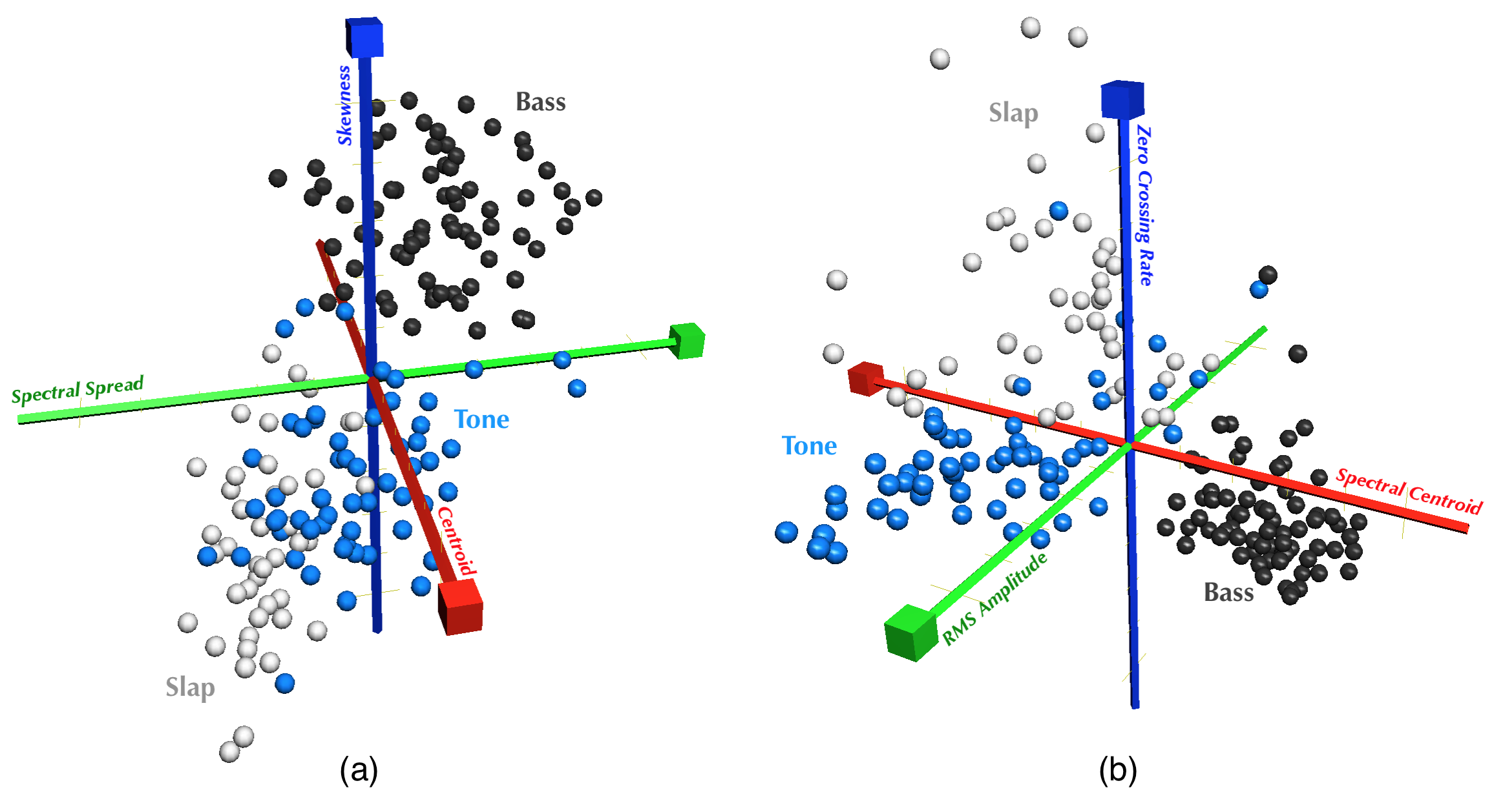
These features alone still leave some overlap in the stroke categories. It was hypothesized that amplitude and noisiness might account for some of this overlap. This was also found to be true, as can be seen in Figure 17 (b), so RMS amplitude and zero-crossing rate were included as features.
All features are normalized across the training set by subtracting the mean and dividing by the standard deviation. This prevents the feature with the largest scale from dominating the classifier.
4.3.3 Realtime Classification
Following [70], a kNN classifier was implemented for the present study. Although the time-complexity of this algorithm is high, it by no means precludes realtime operation in this case. A full analysis is beyond the scope of this paper. Nonetheless, kNN, not including distance calculations, can be implemented to run in O(N) + O(k) time on average (Quicksort by distance, then Quicksort lowest k by category), where N is the number of training examples, k is the number of neighbors, and the symbol O() indicates the order, or upper-bound, of the algorithm's growth-rate as a function of input-size. However, the implementation provided here has a higher complexity in k, and runs in about O(Nk) + O(k2/2). This was tested to run about 10 times faster than the former for values of k < 10, and twice as fast for very high values of k up to 350. This is owing to much simpler `operations' despite a higher time-complexity. In any event, the classifier's accuracy was generally not found to improve for values of k greater than about 5, so the added complexity is small in practice. In both cases, the actual computation time of kNN is dominated by calculating the distances, which has a complexity of O(Nf), where f is the number of features in the model. Because f is fixed by the model, the goal would be to reduce N, which could be done through a variety of techniques, such as clustering. However, even this was not necessary; In practice, the classifier was found to require between about 14 and 32 microseconds to run on a 2.6 GHz Intel i7, for k=5 and N=100. On the other hand, feature calculation, including STFT, required between about 1405 and 2220 microseconds. These calculations can run, at most, every 50 milliseconds (the amount of audio used by this algorithm), which would consume at most about 4% of CPU time. Indeed, the operating system reported the CPU usage of the classifier to be under 7% during a barrage of strokes, and the excess is consistent with the onset-detector's computation time.
4.4 Evaluation
Several experiments were designed to test the classifier's efficacy under a variety of conditions. The first few experiments will go deep and analyze a single instrument, the djembe, in a variety of contexts. Subsequently, a broad assessment of the generalizability of the model will be made by testing it on several instruments. Because in practice it is desirable to capture only the sound of the instrument played by the human, while eliminating the sound of the robot and other extraneous sounds, all instruments in this study are recorded using a piezo-disc contact-mic coupled with a high-impedance amplifier.
4.4.1 The Ecological Case
The first experiment was designed to be simple but ecologically valid, representing how the classifier is intended to be used. A contact-mic was affixed to a djembe. The frequency sensitivity of the mic is highly dependent upon its placement, and a location near the bottom of the drum seemed to capture a good mix of low and high frequencies. Because the curvature of the djembe is not amenable to a flat piezo disc, the disc was coupled to the drum via a small amount of putty. The classifier was trained by playing 20 archetypical examples of each stroke - bass, tone, and slap - in succession. A rhythmic sequence of 125 strokes (49 bass, 47 tone and 30 slap) was then played, and the onset detector and classifier's performance were evaluated. The onset detector correctly identified all onsets and gave no false positives. The classifier was 95% accurate for k=2. The signal data was also recorded and fed back into the classifier for each k from 1 to 5. The worst case was k=5 with accuracy of 86%, as can be seen in Table 2.
| Bass | Tone | Slap | |
| Bass | 41 | 8 | 0 |
| Tone | 0 | 44 | 2 |
| Slap | 0 | 4 | 26 |
The confusion between tone and slap were attributable to the same strokes for each value of k. These strokes were aurally ambiguous to the authors as well. The variation in accuracy as a function of k was attributable to variation in confusion between bass and tone. This is likely due to tie-resolution for ambiguous strokes, which could be improved with a larger training set. It should be noted that leave-one-out cross-validation on the training set indicated very high accuracy: 100% for 1 ≤ k ≤ 3. The lower accuracy on the independent set of observations is probably because strokes used in actual rhythms are somewhat less consistent than their archetypical counterparts, owing to timing constraints, expressive variability, noise in the human motor control system, and the physics of the vibrating drum head.
4.4.2 Loudness
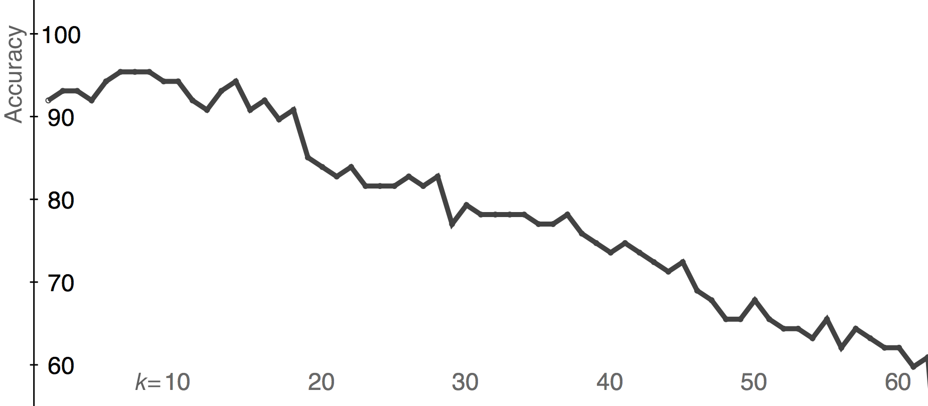
In the previous experiment, the drum was played at a moderate loudness with natural metric accents. Another experiment was conducted to test the accuracy of the classifier when extreme variations in loudness were present. In this experiment, 30 strokes of each category (bass, tone, slap) were recorded on djembe. Of these, 10 were played very softly, 10 intermediate, and 10 very loud. In this case, even after hand-tuning the threshold, the onset detector failed to detect three strokes in the quietest category and spuriously detected two false positives (immediately following a true positive) in the loudest category. The spurious false positives were removed from the data, and no attempt was made to recover the missed strokes. Leave-one-out cross-validation was performed on the data for all values of k, treating them as three stroke categories. The accuracy is slightly improved by choosing k a few greater than 1, and then gradually decreases with increasing k, as can be seen in Figure 18. The classifier was, on average, 93% accurate for 1 ≤ k ≤ 10.
4.4.3 Extended Techniques
Although bass, tone, and slap are the core strokes of djembe technique, skilled players of this and other hand drums define and use many more strokes, which are typically subtler variations on the core three. This experiment tested the classifier's accuracy on a set of 7 strokes: bass, tone, slap, muted slap (dampened with free hand during stroke), closed slap (the striking hand remains on drumhead after stroke), closed bass (ditto) and flam (two quick slaps in rapid succession, taken as a single gestalt). Not all of these are proper to djembe technique, but are characteristic of several Latin American and African instruments. 50 examples of each were played, and cross-validated. The classifier was 90.6% accurate for k=5, and on average 88.2% accurate for for 1 ≤ k ≤ 10. The confusion was as shown in Table 3 for k=4.
| Slap | Tone | Bass | Closed Slap | Muted Slap | Closed Bass | Flam | |
| Slap | 44 | 3 | 0 | 0 | 0 | 0 | 3 |
| Tone | 5 | 45 | 0 | 0 | 0 | 0 | 0 |
| Bass | 0 | 0 | 50 | 0 | 0 | 0 | 0 |
| Closed Slap | 1 | 0 | 0 | 47 | 0 | 0 | 2 |
| Muted Slap | 0 | 0 | 1 | 0 | 46 | 3 | 0 |
| Closed Bass | 0 | 0 | 1 | 2 | 5 | 42 | 0 |
| Flam | 2 | 0 | 0 | 11 | 0 | 0 | 37 |
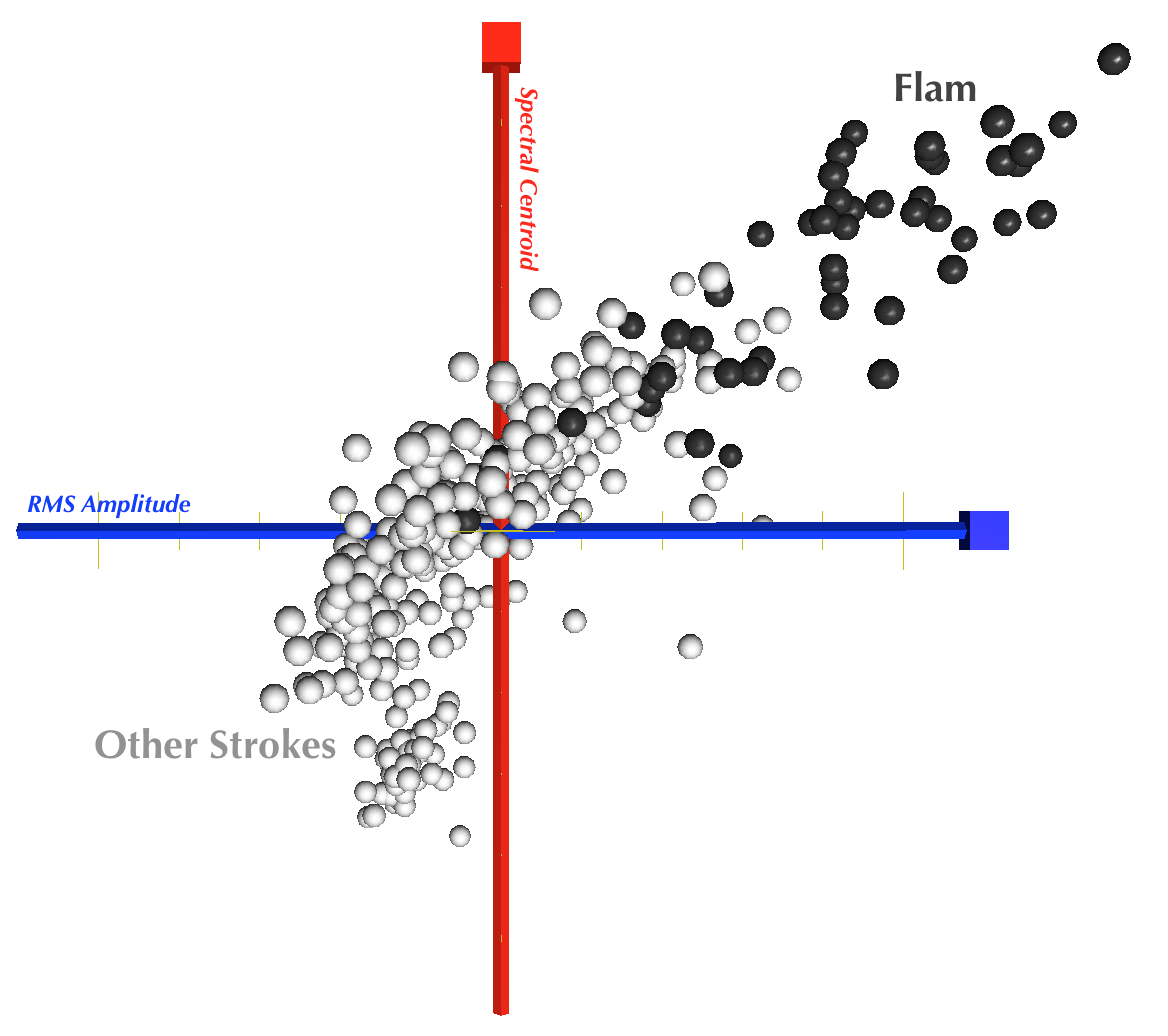
It is interesting to note that the plurality of confusion, 46% of it, involved flam. This was unexpected because flam was hypothesized to contain much more energy over the sample than other strokes, owing to the second attack, which should make it easily identifiable. Although this was true, as is seen in Figure 19, the effect had great variance, which, on the low end, caused many flams to intermingle with the other stroke categories. This is suspected to be a side-effect of the temporal granularity of the onset-detector rather than an acoustic property of the strokes, although further analysis is needed.
4.4.4 Different Instruments
The previous experiments focused on djembe in order to give a complete picture of the classifier's performance on a single instrument. However, the classifier was designed to be more general, so another set of experiments tested several instruments.
4.4.4.1 Cajon
In one experiment, 20 archetypical strokes from each of 4 categories - bass, tone, slap, and muted slap - were played on a Peruvian cajon (wooden box) without snares. Cross-validation revealed an average accuracy of 93% for 1 ≤ k ≤ 10. In another experiment, an uncontrived rhythmic sequence of 168 strokes from three categories was played on cajon. Each stroke was manually labelled (bass, tone, slap) and given to the classifier for analysis. Cross validation on this set yielded an average accuracy of 87% for 1 ≤ k ≤ 10. As with the djembe, the lower accuracy on performed strokes as opposed to contrived ones is likely attributable to greater variability in the acoustic content of the strokes. Generally, archetypical strokes should probably not be used as training examples. Figure 17 depicts this dataset.
4.4.4.2 Darbuka
In this experiment, 30 archetypical strokes from each of 3 categories - doum, tek, and pa - were played on darbuka (ceramic goblet drum). The classifier was on average 96% accurate for 1 ≤ k ≤ 10.
4.4.4.3 Frame Drum
Furthermore, 30 archetypical strokes from each of 3 categories - doum, tek, and pa - were played on a small frame drum (hoop and animal hide) with unusually thick skin. Cross-validation indicated an average of 95% accuracy for 1 ≤ k ≤ 10.
4.4.4.4 Bongos
Several percussion instruments, such as bongos, are actually two separate drums of different pitch, optionally joined together by a center block and bolts. While it would in principle be possible to treat each drum separately, with a separate contact-mic and separate set of training examples for each, in is interesting to know to what extent such instruments could be analyzed as a single unit. Therefore, a contact- mic was placed on the center block joining a pair of bongos. 30 exemplary strokes from each of 5 categories - open and closed strokes on the larger drum, and open, closed, and muted strokes on the smaller drum - were played. Cross validation yielded an average accuracy of 94% for 1 ≤ k ≤ 10. The majority of the confusion was between the open and closed strokes on the larger drum. This is suspected to be due in part to the placement of the contact-mic which was not acoustically ideal but provided a strong signal for both drums. It is hypothesized that the accuracy could be increased by using two separate microphones, one placed directly on the body of each drum. Such microphones could be soldered together in parallel and serviced by a single amplifier and set of classifier training examples.
4.4.5 More Subjects
In the foregoing studies, only one subject, the author, played the percussion instruments. One might therefore argue that the method presented here may not generalize to other subjects. Of course the purpose of using machine learning is that individual subjects can specify their own stroke categories, so it is reasonable to hypothesize that the method will generalize. To test this, three additional subjects with some musical training, only one of whom considers percussion to be a primary instrument, were tested. They were first asked to play 35 archetypical bass, tone, and slap strokes on cajon, as might be done to train the classifier during normal use. Then they were asked to repeat 12 times the rhythm shown in Figure 20. This rhythm was constructed to contain an equal number of strokes in each category, and one of each stroke transition (bass → bass, bass → tone, bass → slap, etc...).

Three tests were performed on this data for each subject. In Test 1, the 105 archetypical strokes in three categories were cross-validated against themselves using leave-one-out cross-validation. In Test 2, the 108 strokes in 12 repetitions of the rhythm were classified using the archetypical strokes as the training set. In Test 3, the 108 strokes in 12 repetitions of the rhythm were cross-validated against themselves.
The classifier's accuracy on these tests are shown in Table 4. The relatively high accuracy on Test 1 accords with data presented elsewhere in this study. It is interesting that Test 3 had a relatively high accuracy compared to Test 2. Test 3 demonstrates that the strokes used in playing are relatively self-consistent, but Test 2 demonstrates that they are not as consistent with the archetypical strokes. This suggests that the subjects' archetypical strokes are not the ones they use in actual playing. It is worth pointing out that all three subjects played the archetypical strokes using only one hand, and the rhythm using both hands. A better training strategy may involve having users play segments of predetermined rhythms. The somewhat lower accuracy of Test 3 compared to Test 1 also accords with data presented elsewhere in this study. It may also be pointed out that subjects universally found the order of the last three strokes in the rhythm confusing. At times they would stop and request to restart the experiment after playing mistakes. This notwithstanding, the final data contains instances where these strokes are, to the author's ears, metathesized. For each subject, these strokes explained a couple of percentage points of the difference between Test 3 and Test 1.
| Subject | Test 1 | Test 2 | Test 3 |
| 1 | 98% | 78% | 94% |
| 2 | 97% | 77% | 90% |
| 3 | 90% | 67% | 84% |
4.5 Conclusion and Future Work
In conclusion, the provided classifier was found to work with relatively high accuracy on a variety of instruments. In practice, its correspondence to human perception is acceptably high for the intended application, i.e. collaborative music making with a musical robot. Future work will use a variant of this algorithm to allow percussion robots to perform auto-calibration. If a human played several archetypical strokes on the instrument as training examples, then the robot could search its control-parameter space (impact angle, velocity, hand tension, etc...) for a point that yielded the lowest self-classification error.
4.6 Acknowledgements
Thanks to Simone Mancuso for generously allowing us to use his instruments. Let us give reverence to the animals whose skin was used in the manufacture of some of the instruments in this study.
4.7 Addendum
After initial publication of this study, and error was found in the algorithm. Section 4.3.2 above explains taking a windowed FFT over a 50 ms sample, and averaging the centroid over the windows. This is not identical to averaging the spectrum over the windows and computing the centroid on that. For abstruse mathematical reasons, the latter should yield better results. Some additional testing shows that the classifier's accuracy increases marginally when using this method. This increase would be more pronounced if the sample were longer or the hop-size smaller.