Chapter 5
TIMBRAL AUTOEVALUATION
Abstract
Human musicians use timbre as an expressive device, selecting those timbres which suit their aesthetic goals. By contrast, robotic musicians tend to play arbitrary timbres defined by limitations in their hardware and software. This paper presents a method whereby musical robots can learn to play particular timbres based on examples provided by human players, thereby making their playing sound more natural and convincing. This could increase the success of musical robots as performers, companions, and therapeutic / rehabilitation devices. Trials of the method presented in the paper show that the robot can find a target timbre in a reasonable amount of time. A perceptual study aimed at linking the robot's performance to human perception is less conclusive, but provides useful insight.5.1 Introduction
For many musical instruments, skillful playing involves the deliberate use of specific timbres. A beginning flautist produces only one timbre, typically all breath and spit; a beginning violinist plays scratchy and squeaky. Virtuosi, by contrast, will navigate the entire timbre space of the instrument, and may elect to play these timbres, but only when it serves their aesthetic goals. Musical robots are frequently designed to use timbre like beginners; they often produce arbitrary timbres rather than specific ones, and these are typically not the canonic timbres used by skilled human players. This paper introduces a method whereby musical robots can learn to produce specific timbres so that they more closely model the playing of skilled humans.
A musical robot will have several control parameters such as, for example, bow pressure and velocity for a violin robot, and there will exist a map between this control space and the instrument's timbre space. However, it can be difficult to make the robot play a particular timbre by manually tuning the control parameters, as these are not generally orthogonal to the timbral features. It would be better if a robot could learn how to produce timbres by listening to examples. If a robot is provided with a target timbre, i.e. by a human playing an example on the robot's instrument, the robot could search for the control parameters that best match the target timbre. It could accomplish this by playing a variety of timbres, listening to itself via a microphone, and using some optimization algorithm to minimize the distance between its own timbre and the target timbre. In this manner, the robot could `learn' technique by example. Moreover, while playing, the ideal control parameters may change if, for example, malfunction or wear changes the strength of actuators or the relative position of components. A suitable optimization algorithm could be run continuously during normal operation, effectively detecting and compensating for these small environmental changes.5.2 Previous Work
A few studies have evaluated striking mechanisms for percussion robots [17][14]. However, these studies have focused on the physical properties of the mechanisms such as impact force and latency, and do not attempt to evaluate the resultant timbres. Seminal work on the Waseda Flutist Robot allows the robot to listen to itself and improve its own intonation and timbre as it plays [3]. This work is based on a previous study that explicitly maps the flute's drive conditions to its timbre space. Since the 1970s, many studies such as [60] have attempted to map the perceptual space of timbral distance by having participants rate the similarity of sounds. In general these have focused on gross differences in timbre between instruments and not on subtleties within a single instrument. There also exist exhaustive lists of signal features related to timbral perception [62]. The author is unaware of any study that deals directly with the challenge at hand, and the present study seeks to synthesize all of these methods to approach a solution.
5.3 Implementation
5.3.1 Control Space
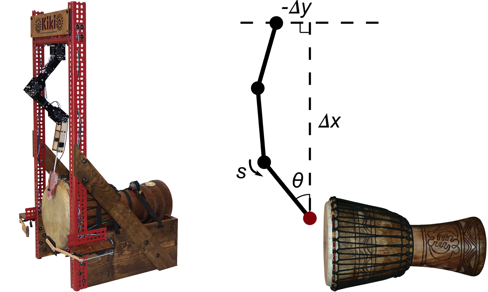
The robot used in this study, Kiki, plays djembe with a 3-DOF arm terminated by a rubber end effector. The word `timbre' comes from the Greek word for drum, and because djembe is unpitched, its playing technique consists primarily in the manipulation of timbre. Kiki's striking algorithm has four control parameters: ∆x, ∆y, θ, and s. These parameters are depicted in Figure 21. ∆x, ∆y and θ specify the strike position. Prior to striking, the arm is moved to a recoil position, which is identical to the strike position except that the most distal servo is rotated away from the drum by some recoil angle. To strike the drum, that servo moves at some angular speed until it reaches the strike location, at which time its power is switched off and it continues moving under inertia. Increasing the parameter s increases both the recoil angle and angular speed. ∆x and ∆y have a resolution of about 1 millimeter, θ has a resolution of approximately 1 milliradian, and s ranges from 0 to 1 in arbitrary units. Not all points in the control space result in the robot actually striking the drum; such points shall be referred to as `invalid'.
5.3.2 Timbre Space
5.3.2.1 Features
Timbral features are extracted from drum strokes as a variation on [64]. Namely, a contact mic is placed on the robot's drum. Stroke onsets are identified when the spectral flux of the incoming audio surpasses a certain threshold. From the note onset, one second of audio is recorded. Note that in the current study it is not necessary to choose a shorter duration to accommodate the fast repetition rates found in natural playing. Two features, RMS amplitude and zero-crossing rate (ZCR), are extracted from this sample. Additionally, a windowed DFT is taken over the sample and averaged over the windows. Four additional features, the first four spectral moments - centroid, spread, skewness, kurtosis - are calculated on the averaged spectrum. Timbral comparisons shall be made using Euclidian distance on these six features. However, these features all have different scales, so the feature with the largest scale would dominate the distance calculation. In order to determine the relative scales of the features, the timbre space must be sampled by playing many arbitrary strokes of different timbres on the drum. This shall be referred to as `normalizing the timbre space', and can be done efficiently by a human or robot. The software then calculates and stores the arithmetic mean and standard deviation of each feature across the samples. Subsequently, all samples are mapped from the raw feature space to the scaled feature space by normalization, i.e. each observed raw feature has its mean subtracted from it, and is divided by its standard deviation. For the remainder of this paper, all operations shall be performed in the scaled space.
5.3.2.2 Expected Distances
The goal of this paper is to minimize the distance between the robot's timbre and some target timbre, but how close are two randomly selected timbres expected to be, and what distance constitutes significantly smaller than random? To answer this, the distribution of distances in the timbre space must be analyzed. Let it be assumed that the timbral features are independent and timbres are normally distributed in each feature. Consider two n-dimensional feature vectors, x and y. The square of their distance, r2 is given by r2 = zTz, where z = x − y and T represents matrix transposition. What is the distribution of z? In general, the distribution of the difference of two normally distributed variables x ∼ N(μx, σ2x) and y ∼ N(μy, σ2y) is another normally distributed variable z ∼ N(μz, σ2z) where μz = μx − μy and σ2z = σ2x + σ2y. In the n-dimensional case, if the features have the same variance and are not correlated, this will generalize as z ∼ N(μz, σ2zI), where where I denotes the identity matrix. Thus, in the present case, because the features are normalized and assumed independent, z has zero mean and covariance matrix 2I, i.e. z ∼ N(0, 2I). The probability density function of r2 given this distribution of z is solved in [75]. It is a gamma distribution Γ(α, β) with parameters α = [n/2] and β = 2σ2z,
| (1) |
| (2) |
| (3) |
| (4) |
That defines an upper bound on how close learned timbres should be. What about a lower bound? How close must two timbres be to be considered identical? To assess this, the robot Kiki was asked to strike the drum 25 times using exactly the same striking method each time, and the timbral distances were calculated (note that there are 300 distances between 25 strokes). This process was performed for three striking methods, and the results are shewn in Table 5. The results are tightly clustered in the timbre space for each striking method. According to this distances less than about 0.1 may be considered roughly identical.
| Striking Method | Mean Distance | Variance |
| 1 | 0.0748 | 0.0028 |
| 2 | 0.1162 | 0.0069 |
| 3 | 0.0368 | 0.0011 |
5.3.3 Map
Insofar as the goal is to explore the map from the control space onto the timbre space, it is useful to identify some properties that the map may or may not possess. First, it should not be assumed, based on prior knowledge, that particular points in the control space will map to particular points in the timbre space. For example, humans make a resonant bass sound by striking the center of the djembe, but since the robot's body is not identical to a human's, it may produce the same timbre with an unexpected striking method. Moreover, the map should be assumed to be neither surjective nor injective. The former admits that there may exist regions of the timbre space that are not reachable by the robot. The latter admits that two different striking methods may produce the same timbre. One may be tempted to evaluate the robot's ability to find a timbre using striking method as a proxy; the robot could play a target timbre using a known striking method, then, after searching for the target timbre, the resulting striking method could be compared to the original one. However, non-injectivity asserts that the robot's inability to find the original striking method does not imply that it has not found the original timbre. In this study, the map will be assumed to be continuous, such that adjacent striking methods produce adjacent timbres.
5.3.4 Optimization
Because the map between between the control and timbre spaces is unknown, an optimization algorithm is used to search for the global minimum between two timbres. In the current study, a variation on simulated annealing was used. This works as follows.
- The timbre space is normalized with many arbitrary strokes.
- A target timbre, ttarget, is defined (i.e. the human plays a target stroke on the robot's drum).
- A variable known as the `most recently accepted striking method', caccepted, is defined.
- caccepted must be initialized to a striking method that is known to be valid. The robot strikes the drum with this method, calculates the timbral features, and measures the Euclidian distance, raccepted, to ttarget in the timbre space.
- A new candidate striking method, ccandidate is generated by starting with caccepted, randomly selecting one feature in the control space, and nudging it up or down by a random amount within certain range. The ranges are proportional to the annealing temperature, T, which is reduced with each successive iteration of this step.
- The robot strikes the drum using ccandidate. If this stroke is not valid, ccandidate is unconditionally rejected. If it is valid, the Euclidian distance, rcandidate, to ttarget is calculated. ccandidate will be accepted with a probability of eraccepted − rcandidate / T. Accepting a stroke means setting caccepted ← ccandidate.
- Steps 5 and 6 are iterated for many generations. If they are iterated more than a certain number of times without producing a candidate stroke that is closer to ttarget than the closest candidate thus far, cbest, then caccepted ← cbest.
- cbest is returned. cbest should, in principal, be caccepted, but might not be if the algorithm has moved out of the region of the global minimum and has become temporarily stuck in the vicinity of some local minimum. cbest is not likely to have been produced in the last generation.
5.4 Evaluation
4 Evaluation
Two types of evaluation are performed for this technique. First, computational methods shall be used used to ascertain the algorithm's success in reaching a target point in the timbre space. Secondly, a perceptual study determines whether the algorithm becomes perceptually closer to the target as it runs.5.4.1 Computational
5.4.1.1 Trials
This algorithm was run a number of times and its performance evaluated. The algorithm was normalized using the 600 strokes recorded in Section 5.4.2 below - 400 robot strokes and 200 human strokes. T started at 1 and was reduced by 10% at each generation. New features were generated with bounds ±50T mm for ∆x, ±10T mm for ∆y, ±50T milliradians for θ, and ±0.5T units for s. caccepted was replaced with cbest after 10 successive candidates worse than cbest.
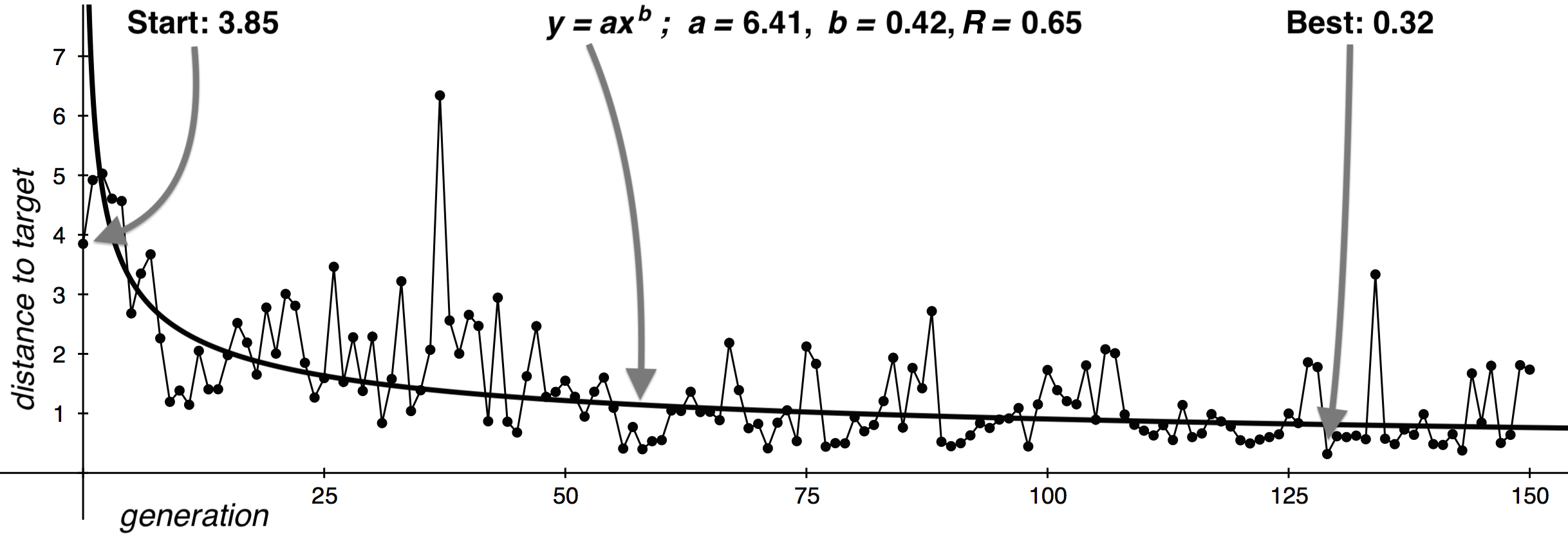
The robot started each trial run with a tone-like stroke and proceeded for 150 generations. The robot takes 600 milliseconds to strike the drum before recording 1 second of audio, so one run takes about 4 minutes. For each target stroke, the algorithm was run three times using that identical target. This process was carried out for a bass, tone, and slap target, resulting in 9 trial runs. The starting and ending (i.e. best) distances were recorded for each run. Additionally, the distance of each candidate stroke to the target was recorded, a curve of the form y=axb was fitted to this data using a power regression model, and the Pearson Correlation coefficient, R, was calculated for the regression. For clarity, these variables are depicted in Figure 22 for trial 9. Additionally, the results of all 9 trials are shown in Table 6.
| Trial | Target | Start | End | a | b | R |
| 1 | tone | 1.54 | 0.29 | 2.45 | -0.22 | 0.13 |
| 2 | tone | 1.82 | 0.42 | 2.20 | -0.13 | 0.11 |
| 3 | tone | 2.02 | 0.47 | 1.64 | -0.03 | 0.21 |
| 4 | bass | 4.53 | 2.78 | 5.80 | -0.10 | 0.52 |
| 5 | bass | 4.98 | 2.08 | 5.08 | -0.09 | 0.45 |
| 6 | bass | 5.42 | 1.89 | 7.32 | -0.24 | 0.73 |
| 7 | slap | 3.04 | 0.54 | 6.05 | -0.32 | 0.41 |
| 8 | slap | 4.20 | 0.42 | 2.81 | -0.20 | 0.31 |
| 9 | slap | 3.85 | 0.32 | 6.41 | -0.42 | 0.65 |
5.4.1.2 Trends
In each trial, the signs of the coefficients a and b, positive and negative respectively, indicate a trend of decreasing distance eventually converging on 0. For bass and slap targets, this trend is highly significant with p < 0.001. For tone targets, the trend is, in general, scantly significant; this is to be expected because the algorithm started with a tone-like stroke relatively close to the target. In this case, one would expect the regression curve to have nearly 0 slope, which will have 0 significance for any data. Note that this does not prevent the algorithm from ending much closer to the target than where it started; it only means that the algorithm did not perform much better than playing random strokes and picking the best. This is not surprising because that is the basic principal of operation behind simulated annealing. In these cases, the algorithm would probably converge faster if the search space for new candidate striking methods were proportional to raccepted and not just T, which would reduce the variance thereby increasing the significance. This would also increase the likelihood that the algorithm would become trapped in a suboptimal local minimum.
5.4.1.3 Unreachability
For tone and slap targets, the algorithm finished very near the target. For the bass target, although the algorithm became significantly closer to the target, it ended somewhat far away. Evidently the target was in an unreachable region of the timbre space. In particular, in these trials, many strokes were rejected as invalid, and this occurred for two reasons. Some candidates contained the lowest value of s producible by the robot, or nearly so, and many of these were too quiet to trip the onset detector. Second, these trials resulted in the robot's arm fully extended with nearly maximum values of ∆x, and many stroke candidates were out of the arm's reach. These trials were repeated for the same target after lowering the onset detector's threshold and physically lowering the arm with respect to the drum. While this decreased the number of rejected strokes, it did not improve the best distance. To the author's ear, in all trials with a bass target, the algorithm did converge on what sounded like passable bass strokes, albeit quieter and less resonant than the target. Raising s would have made the stroke louder, but would have changed the spectral distribution in a way that evidently could not be compensated by the other control parameters. For all trials with slap and tone targets, the result did sound to the researcher to be quite similar to the target, but after listening to 150 intervening candidate strokes it is difficult to make a nuanced comparison, which generally prohibits a more rigorous perceptual evaluation of an entire trial run taken as a unit.
These trials all started with a tone-like stroke as the first candidate. In practice, it may be better to store a list of many striking methods and their approximate timbres, and select from that list a starting candidate that is already close to the target. In many cases, this would help the algorithm find good strokes in fewer steps.
5.4.2 Perceptual
The previous section demonstrates that the proposed algorithm successfully approaches a target timbre in the timbre space. It does not demonstrate that accepted candidate strokes become perceptually closer to the target as the algorithm runs. The observation that the feature set can be used to classify strokes, as presented in Chapter 4, provides evidence that broad regions of the timbre space do correspond to perception. Similarly, the observation that identical striking methods are tightly clustered in the timbre space provides evidence that the space corresponds to perception at a very local level. Furthermore, some of the timbral features are already known to relate to perception of timbral similarity; for example [60] finds perceptual brightness to be important in how humans determine timbral similarity, and spectral centroid is known to be a correlate of brightness. What about the specific case in which arbitrary robot strokes are compared to an arbitrary human stroke, as is performed at each generation of the algorithm?
5.4.2.1 Methodology
The following experiment was designed to test this. First a large list of random striking methods was generated and invalid methods were manually removed, resulting in 416 methods. Human participants with at least some musical training were asked to listen to the researcher play an arbitrary stroke S on the robot's drum. Then the robot played two strokes, A and B, chosen randomly from the list. The subject was asked to assess which of the robot's strokes, A or B, sounded most similar to S . The subjects were given 5 choices: A was much more similar than B to S; A was slightly more similar; equally similar; B was slightly more similar than A; B was much more similar. These responses were coded as the integers 1 to 5, respectively. This was repeated 50 times for each of 4 subjects. The strokes were also recorded through a contact-mic placed on the body of the drum and later played back into the robot's listening system. For each subject, the timbre space was normalized with all 150 strokes played during the trial. The robot also rated the relative similarity of A and B to S according to dist(A, S) − dist(B, S) where dist() is the Euclidian distance in the timbre space. The robot's responses were cross-correlated with the humans'. Results are shown in Table 7.
| Subject | R (6 features) | R (4 MFCCs) | Experience |
| all | 0.39 | 0.33 | |
| 1 | 0.57 | 0.53 | doctorate in music |
| 2 | 0.49 | 0.48 | masters in music |
| 3 | 0.37 | 0.36 | no music degrees, teaches music professionally |
| 4 | 0.20 | 0.06 | no music degrees, avocational music experience |
5.4.2.2 Listening Styles
The humans' responses, taken all together, were only moderately correlated with the robot's, but the correlation was highly significant (N=200, R=0.392739, p < 0.001). When the analysis is performed separately for each subject, it is seen that the robot agrees more strongly with subjects that have more academic musical training. The robot's agreement is significant for participants 1, 2, and 3 with p < 0.01, and not significant for participant 4 with p < 0.2. From this it does not necessarily follow that the robot more strongly models `expert' listeners, or that low correlation indicates faulty listening; participant 4 is also the only one that claims percussion as a primary instrument, and that individual may have a different style of listening than is modeled here. To attempt to unravel the role of listening style, the analysis was repeated for all 62 combinations of the 6 features. For subjects 1, 2, and 3, spectral centroid alone predicted their responses at least as well as the full set of features. By contrast, participant 4's responses were completely uncorrelated with centroid, but RMS amplitude alone predicted their responses better than the full set of features. The participants were also asked to define the word `timbre', and to an extent their responses confirm these observations. Participants 2 and 3 both provided definitions based on the spectral content of sound: "Timbre is the unique frequency content of a particular sound...", and "Timbre is ... related to the specific harmonic spectra that make up a sound." Participant 4, by contrast, resisted a purely spectral definition, saying that timbre is "not necessarily pitch, but it would be more the warmth or the coldness of the sound." Subject 1's response was more enigmatic: "Usually when you talk about timbre you are talking about the color of the sound, in a sense. Variation in color." It may be the case that some listeners have been trained to listen specifically to spectral features, so naturally those features predict the responses of those individuals better than other individuals.
5.4.2.3 Controls
Based on these results, it is reasonable to wonder whether the robot is better at predicting relative perceptual distances when the absolute perceptual distances are small. Perhaps when A and B are both perceptually very dissimilar to S, the degree of dissimilarity becomes difficult to assess, resulting in more-random responses. Unfortunately, absolute perceptual distances were not collected in this study.
5.4.2.4 Other Features
Are there other features that would be better predictors of the participant's responses? The above analysis was repeated for all combinations of the first 13 Mel Frequency Cepstral Coefficients (MFCCs), calculated with 24 Mel bands, instead of the original 6 features. The first four MFCCs, including the 0th, performed slightly worse than the original 6 features, and adding more coefficients generally reduced the robot's agreement with participants. These results are also shown in Table 7. Participants were asked to provide adjectives describing the timbre of djembe, as well as the timbre of individual djembe strokes relative to one-another. Several responses corresponded to the features used in this study: "deep", "higher pitched", "the rimshot stroke seems to have very strong high partials", "bright", "bassy to trebbly", "high and low". Other features not used in this study, such as the shape of the amplitude envelope and the temporal evolution of the spectrum, are also know to be important in how humans compare timbres. Some of the participants' responses corresponded to these features, and others still were more enigmatic: "visceral", "embodied [the bass stroke]", "there is a whole range between more resonant strokes and kind of clipped", "like a stomp almost ... you can feel that in your foot", "quick attack", "It could thump", "warm", "percussive", "snappy", "accented and unaccented", "piercing", "woody", "natural", "clean". The addition of temporal centroid did not significantly improve the results, which is perhaps not surprising in the case of the djembe, which is not a sustaining instrument. Perhaps other features may increase the agreement between robot and humans.
5.5 Discussion
Although the results in Section 5.4.1 suggest the algorithm can find target timbres, whether those results correspond to perception is less conclusive. The foregoing analysis suggests that listeners will only sometimes agree with the robot at a given generation of the algorithm, and listeners will only sometimes agree with one-another about whether they agree with the robot; there may exist no Truth about this algorithm's success from a perceptual standpoint. On the other hand, the perceptual difference between timbres in this study were all very subtle, and it is possible that the results owe to inconsistent responses within each participant. Nonetheless, the regressions depicted in Figure 22 suggests that the robot will eventually converge on a timbre that is `identical' to the target (given that the target is reachable), according to the definition of `identical' in Table 5. Additionally the observations in Section 5.4.2 suggest that `identical' will correspond to perception in cases when temporal features play a minimal role. It is likely that this model overfits the djembe, and trials should be run on other robots, particularly those that play sustaining instruments. This might assist the development of a more robust feature set that more closely models more listeners and instruments, which in turn would help more musical robots sound more like skilled musicians when they play.